Performance Issues
A major goal of xmitgcm is to achieve scalable performance with very large datasets. We were motivated by the new LLC4320 simulations run by Dimitris Menemenlis and Chris Hill on NASA’s Pleiades supercomputer.
This page documents ongoing research into the performance of xmitgcm.
LLC Reading Strategies
The physical layout of the LLC MDS files creates a challenge for performance. Some of the cube facets are written with C order, while others are written with Fortran order. This means that complex logic is required to translate the raw data on disk to the desired logical array layout within xarray. Because of this complication, the raw data cannot be accessed using the numpy ndarray data model.
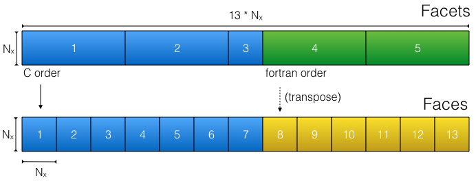
The physical layout of a single level of LLC data in terms of facets (top) and the translation by xmitgcm to faces (bottom).
Two different approaches to reading LLC data have been developed. This option
is specified via the llc_method keyword in open_mdsdataset.
smallchunks
method="smallchunks" creates a large number of small dask chunks to
represent the
array. A chunk (of size nx x nx) is created for each face of each vertical
level. The total number of chunks is consequently 13 * nz. This appears
to perform better when you want to access a small subset of a very large model,
since only the required data will be read. It has a much lower memory footprint
than bigchunks. No memmaps are used withsmallchunks, since that implies leaving
a huge number of files open. Instead, each chunk is read directly by
numpy.fromfile.
bigchunks
method="bigchunks" loads the entire raw data on disk as either a
numpy.memmap (default) or directly as a numpy array. It then slices this
array into facets, reshapes them as necessary, slices each facet into faces,
and concatenates the faces along a new dimension using
dask.array.concatentate. This approach can be more efficient if the goal is
to read all of the array data into memory. Any attempt to read data from the
reshaped faces (faces 8-13 in the cartoon above) will trigger the
entire facet to be loaded into memory. For this reason, the bigchunks method
is impractical for very large LLC datasets that don’t easily fit into memory
comparison
A test script
was developed to evaluate the two strategies for reading LLC4320 data on
Pleiades. Files were selected for analysis randomly from over 10000 files on
disk in order to avoid any caching from the filesystem. The data were read
using the low level routine read_3d_llc_data (see Low Level Utilities). Tests
were performed on both 2D data (4320 x 56160 32-bit floats) and 3D data
(4320 x 56160 x 90 32-bit floats).
The first task was a reduction: computing the sum of the array. For 2D data, the smallchunks method performed marginally better in terms of speed and memory usage.
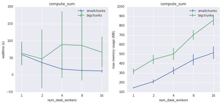
Walltime and memory usage for compute_sum on 2D data as a function of
number of dask workers
However, a dramatic difference was evident for 3D data. The inefficient memory usage of bigchunks is especially evident for large numbers of dask workers, since each worker repeatedly triggers the loading of whole array facets.
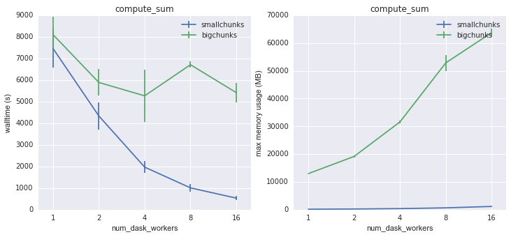
Walltime and memory usage for compute_sum on 3D data as a function of
number of dask workers
For this sort of reduction workflow, smallchunks with a large number of dask workers is the clear winner.
A second common workflow is subsetting. In the test script, we load into memory 1080 x 1080 region from chunk 2.
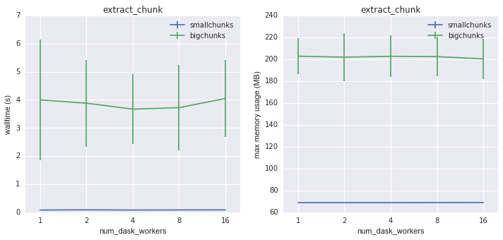
Walltime and memory usage for extract_chunk on 2D data as a function of
number of dask workers
Again, smallchunks is the clear winner here, with much faster execution and lower memory usage. Interestingly, there is little speedup using multiple multiple workers. All the same conclusions are true for 3D data.
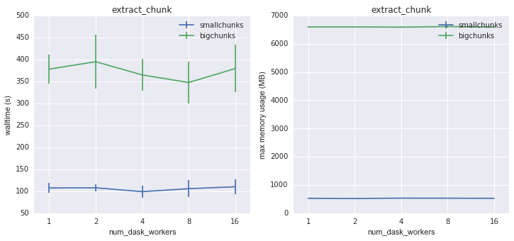
Walltime and memory usage for extract_chunk on 3D data as a function of
number of dask workers
A final workload is simply loading the whole array into memory. (This turned out to be impossible for 3D data, since the compute nodes ran out of memory in the process.) This is the only workload where bigchunks has some advantages. Here a tradeoff between speed and memory usage is clear: bigchunks goes faster because it reads the data in bigger chunks, but it also uses much more memory.
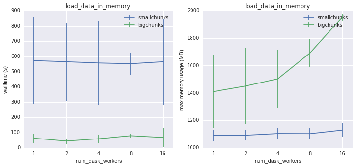
Walltime and memory usage for load_data_in_memory on 2D data as a
function of number of dask workers
It is useful to compare these numbers to the speed of a raw numpy.fromfile
read of the data. This measures the overhead associated with chunking and
reshaping the data from its physical layout on disk to the desired logical
layout. Reading with smallchunks takes about 150 times the raw read time, while
for bigchunks it is more like 10 times. Here there is a disadvantage to using
multiple dask workers; while there is no speed improvement, the memory usage
increases with number of workers for bigchunks.
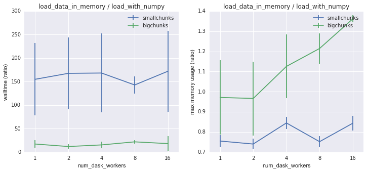
Walltime and memory usage for load_data_in_memory on 2D data as a
function of number of dask workers, normalized against loading the same
data directly using numpy.fromfile.
Running xmitgcm on Pleaides
These instructions describe how to get a working xmitgcm environment on a cluster such as Pleiades. (See related blog post)
Step 1: Install miniconda in user space
Miniconda is a mini version of Anaconda that includes just conda and its dependencies. It is a very small download. If you want to use python 3 (recommended) you can call:
wget https://repo.continuum.io/miniconda/Miniconda3-latest-Linux-x86_64.sh -O miniconda.sh
or for python 2.7:
wget https://repo.continuum.io/miniconda/Miniconda2-latest-Linux-x86_64.sh -O miniconda.sh
Step 2: Run Miniconda
Now you actually run miniconda to install the package manager. The trick is to specify the install directory within your home directory, rather in the default system-wide installation (which you won’t have permissions to do). You then have to add this directory to your path:
bash miniconda.sh -b -p $HOME/miniconda export PATH="$HOME/miniconda/bin:$PATH"
Step 3: Create a custom conda environment specification
You now have to define what packages you actually want to install. A good way to do this is with a custom conda environment file. The contents of this file will differ for each project. Below is an environment.yml suitable for xmitgcm:
name: xmitgcm
dependencies:
  - numpy
  - scipy
  - xarray
  - netcdf4
  - dask
  - jupyter
  - matplotlib
  - pip:
    - pytest
    - xmitgcm
Create a similar file and save it as environment.yml.
Step 4: Create the conda environment
You should now be able to run the following command:
conda env create --file environment.yml
This will download and install all the packages and their dependencies.
Step 5: Activate The environment
The environment you created needs to be activated before you can actually use it. To do this, you call:
source activate xmitgcm
This step needs to be repeated whenever you want to use the environment (i.e. every time you launch an interactive job or call python from within a batch job).
Step 6: Use xmitgcm
You can now call ipython on the command line or launch a jupyter notebook and import xmitgcm. This should be done from a compute node, rather than the head node.
Example Pleiades Scripts
Below is an example python which extracts a subset from the LLC4320 simulation on Pleiades and saves it a sequence of netCDF files.
import os
import sys
import numpy as np
import xarray as xr
import dask
from multiprocessing.pool import ThreadPool
from xmitgcm import open_mdsdataset

# By default, dask will use one worker for each core available.
# This can be changed by uncommenting below
#dask.set_options(pool=ThreadPool(4))

# where the data lives
data_dir = '/u/dmenemen/llc_4320/MITgcm/run/'
grid_dir = '/u/dmenemen/llc_4320/grid/'
# where to save the subsets
outdir_base = '/nobackup/rpaberna/LLC/tile_data/'

dtype = np.dtype('>f4')

# can complete 300 files in < 12 hours
nfiles = 300

# the first available iteration is iter0=10368
# we start from an iteration number specified on the command line
iter0 = int(sys.argv[1])

delta = 144 # iters
delta_t = 25. # seconds
all_iters = iter0 + delta*np.arange(nfiles)

region_name = 'agulhas'
region_slice = {'face': 1,
                'i': slice(1080,3240), 'i_g': slice(1080,3240),
                'j': slice(0,2160), 'j_g': slice(0,2160)}

fprefix = 'llc_4320_%s' % region_name
outdir = os.path.join(outdir_base, fprefix)

ds = open_mdsdataset(data_dir, grid_dir=grid_dir,
                     iters=list(all_iters), geometry='llc', read_grid=False,
                     default_dtype=np.dtype('>f4'), delta_t=delta_t,
                     ignore_unknown_vars=True)

region = ds.isel(**region_slice)

# group for writing
iters, datasets = zip(*region.groupby('iter'))
paths = [os.path.join(outdir, '%s.%010d.nc' % (fprefix, d))
         for d in iters]

# write the data...takes a long time and executes in parallel
xr.save_mfdataset(datasets, paths, engine='netcdf4')
Here is a batch job which calls the script
#!/bin/bash
#PBS -N read_llc
#PBS -l select=1:ncpus=28:model=bro
#PBS -l walltime=12:00:00

source activate xmitgcm
cd $PBS_O_WORKDIR
# the first available iteration
iter0=10368
python -u write_by_iternum.py $iter0