llcreader
This module provides optimized routines for reading LLC data from disk or over the web, via xarray and dask. This was motivated explicitly by the need to provide easy access to the NASA-JPL LLC4320 family of simulations, in support of the NASA SWOT Science Team.
Warning
These routines are new and experimental. APIs are subject to change.
Eventually the functionality provided by llcreader may become part of
the main xmitgcm module.
Limitations
llcreader uses Dask to provide a lazy view of the data; no data are actually loaded into memory until required for computation. The data are represented using a graph, with node corresponding to a specific chunk of the full array. Because of the vast size of the LLC datasets, the user is advised to read about Dask best practices. If you wish to work with the full-size datasets, you must be aware of Dask’s inherent limitations, and first gain experience with smaller problems. In particular, it is quite easy to create very large Dask graphs that can overwhelm your computer’s memory and CPU capacity, even without loading any data!
To make this warning more concrete, let’s consider a single variable such as
Theta from the LLC4320 simulation.
In “face” form, the dimensions of this array are 9030 timesteps x 90 vertical
levels x 13 faces x 4320 j points x 4320 i points = 197170122240000 values.
With 32-bit precision, this requires 788 TB of memory!
If we divide this array into 1 GB chunks, we will have 788,000 chunks.
The lazy representation of the array requires about 1 kB of memory per chunk,
and processing the graph for computation requires about 200 µs per chunk.
Therefore, the lazy representation will occupy nearly 1GB of memory and take
nearly 3 minutes to even begin computation.
There are 5 such 3D variables in the LLC4320 dataset, plus another 10 2D
variables.
The bottom line is that creating graphs of this size will seriously bog down
a laptop.
There are several strategies that can be used to mitigate this problem:
Subset variables: llc reader allows you to create datasets the contain only the specific variables you need, via the
varnameskeyword.Subset vertical levels: if you don’t need full depth fields, you can select just the depth levels you need using the
k_levelskeyword.Subset in time: you can specific the iteration number start, stop and step manually.
Use larger chunks: llcreader allows you to vary the size of the chunks in the
kdimension using thek_chunksizekeyword. Using full depth chunks (k_chunksize=90) will produce chunks up to 20 GB in size, but in a much smaller graph.
Because of how the files are compressed and stored on disk, unfortunately it is not possible to subset in space at the time of dataset creation. However, this can be done later, via xarray.
Pre-Defined Models
We provide some pre-defined references to existing stores and models that can be used right away. These are
llcreader.ECCOPortalLLC2160Model: LLC2160 accessed via ECCO data portalllcreader.ECCOPortalLLC4320Model: LLC4320 accessed via ECCO data portalllcreader.PleiadesLLC2160Model: LLC2160 accessed on Pleaides filesystemllcreader.PleiadesLLC4320Model: LLC4320 accessed on Pleaides filesystemllcreader.CRIOSPortalASTE270Model: ASTE Release 1 accessed via AWSllcreader.SverdrupASTE270Model: ASTE Release 1 accessed on Sverdrup filesystem at UT Austin
Below are a few examples of how to use these.
ECCO HTTP Data Portal
NAS has created an experimental data portal to access the LLC data over the
web via standard HTTP calls.
More info and a data browser can be found at
https://data.nas.nasa.gov/ecco/.
The llcreader module provides a way to access this data directly via
xarray and dask.
These examples can be run from anywhere; however the speed at which data can
be loaded depends on the network bandwidth to the NAS HTTP server and the
rate at which this server can extract data from the underling filesystem.
In this example, we display the whole dataset lazily, following the advice above
to use a large k_chunksize.
By default, all variables and all timesteps are loaded:
>>> from xmitgcm import llcreader
>>> model = llcreader.ECCOPortalLLC4320Model()
>>> ds = model.get_dataset(k_chunksize=90)
>>> print(ds)
<xarray.Dataset>
Dimensions:   (face: 13, i: 4320, i_g: 4320, j: 4320, j_g: 4320, k: 90, k_l: 90, k_p1: 91, k_u: 90, time: 9030)
Coordinates:
  * face      (face) int64 0 1 2 3 4 5 6 7 8 9 10 11 12
  * i         (i) int64 0 1 2 3 4 5 6 7 ... 4313 4314 4315 4316 4317 4318 4319
  * i_g       (i_g) int64 0 1 2 3 4 5 6 7 ... 4313 4314 4315 4316 4317 4318 4319
  * j         (j) int64 0 1 2 3 4 5 6 7 ... 4313 4314 4315 4316 4317 4318 4319
  * j_g       (j_g) int64 0 1 2 3 4 5 6 7 ... 4313 4314 4315 4316 4317 4318 4319
  * k         (k) int64 0 1 2 3 4 5 6 7 8 9 10 ... 80 81 82 83 84 85 86 87 88 89
  * k_u       (k_u) int64 0 1 2 3 4 5 6 7 8 9 ... 80 81 82 83 84 85 86 87 88 89
  * k_l       (k_l) int64 0 1 2 3 4 5 6 7 8 9 ... 80 81 82 83 84 85 86 87 88 89
  * k_p1      (k_p1) int64 0 1 2 3 4 5 6 7 8 9 ... 81 82 83 84 85 86 87 88 89 90
    niter     (time) int64 ...
  * time      (time) datetime64[ns] 2011-09-13 ... 2012-09-23T05:00:00
    drC       (k_p1) >f4 dask.array<chunksize=(91,), meta=np.ndarray>
    drF       (k) >f4 dask.array<chunksize=(90,), meta=np.ndarray>
    dxC       (face, j, i_g) float32 dask.array<chunksize=(3, 4320, 4320), meta=np.ndarray>
    dxF       (face, j, i) float32 dask.array<chunksize=(3, 4320, 4320), meta=np.ndarray>
    dxG       (face, j_g, i) float32 dask.array<chunksize=(3, 4320, 4320), meta=np.ndarray>
    dyC       (face, j_g, i) float32 dask.array<chunksize=(3, 4320, 4320), meta=np.ndarray>
    dyF       (face, j, i) float32 dask.array<chunksize=(3, 4320, 4320), meta=np.ndarray>
    dyG       (face, j, i_g) float32 dask.array<chunksize=(3, 4320, 4320), meta=np.ndarray>
    hFacC     (k, face, j, i) float32 dask.array<chunksize=(90, 3, 4320, 4320), meta=np.ndarray>
    hFacS     (k, face, j_g, i) float32 dask.array<chunksize=(90, 3, 4320, 4320), meta=np.ndarray>
    hFacW     (k, face, j, i_g) float32 dask.array<chunksize=(90, 3, 4320, 4320), meta=np.ndarray>
    PHrefC    (k) >f4 dask.array<chunksize=(90,), meta=np.ndarray>
    PHrefF    (k_p1) >f4 dask.array<chunksize=(91,), meta=np.ndarray>
    rA        (face, j, i) float32 dask.array<chunksize=(3, 4320, 4320), meta=np.ndarray>
    rAs       (face, j_g, i) float32 dask.array<chunksize=(3, 4320, 4320), meta=np.ndarray>
    rAw       (face, j, i_g) float32 dask.array<chunksize=(3, 4320, 4320), meta=np.ndarray>
    Z         (k) >f4 dask.array<chunksize=(90,), meta=np.ndarray>
    Zp1       (k_p1) >f4 dask.array<chunksize=(91,), meta=np.ndarray>
    rhoRef    (k) >f4 dask.array<chunksize=(90,), meta=np.ndarray>
    XC        (face, j, i) float32 dask.array<chunksize=(3, 4320, 4320), meta=np.ndarray>
    YC        (face, j, i) float32 dask.array<chunksize=(3, 4320, 4320), meta=np.ndarray>
    Zl        (k_l) >f4 dask.array<chunksize=(90,), meta=np.ndarray>
    Zu        (k_u) >f4 dask.array<chunksize=(90,), meta=np.ndarray>
Data variables:
    Eta       (time, face, j, i) float32 dask.array<chunksize=(1, 3, 4320, 4320), meta=np.ndarray>
    KPPhbl    (time, face, j, i) float32 dask.array<chunksize=(1, 3, 4320, 4320), meta=np.ndarray>
    oceFWflx  (time, face, j, i) float32 dask.array<chunksize=(1, 3, 4320, 4320), meta=np.ndarray>
    oceQnet   (time, face, j, i) float32 dask.array<chunksize=(1, 3, 4320, 4320), meta=np.ndarray>
    oceQsw    (time, face, j, i) float32 dask.array<chunksize=(1, 3, 4320, 4320), meta=np.ndarray>
    oceSflux  (time, face, j, i) float32 dask.array<chunksize=(1, 3, 4320, 4320), meta=np.ndarray>
    oceTAUX   (time, face, j, i_g) float32 dask.array<chunksize=(1, 3, 4320, 4320), meta=np.ndarray>
    oceTAUY   (time, face, j_g, i) float32 dask.array<chunksize=(1, 3, 4320, 4320), meta=np.ndarray>
    PhiBot    (time, face, j, i) float32 dask.array<chunksize=(1, 3, 4320, 4320), meta=np.ndarray>
    Salt      (time, k, face, j, i) float32 dask.array<chunksize=(1, 90, 3, 4320, 4320), meta=np.ndarray>
    SIarea    (time, face, j, i) float32 dask.array<chunksize=(1, 3, 4320, 4320), meta=np.ndarray>
    SIheff    (time, face, j, i) float32 dask.array<chunksize=(1, 3, 4320, 4320), meta=np.ndarray>
    SIhsalt   (time, face, j, i) float32 dask.array<chunksize=(1, 3, 4320, 4320), meta=np.ndarray>
    SIhsnow   (time, face, j, i) float32 dask.array<chunksize=(1, 3, 4320, 4320), meta=np.ndarray>
    SIuice    (time, face, j, i_g) float32 dask.array<chunksize=(1, 3, 4320, 4320), meta=np.ndarray>
    SIvice    (time, face, j_g, i) float32 dask.array<chunksize=(1, 3, 4320, 4320), meta=np.ndarray>
    Theta     (time, k, face, j, i) float32 dask.array<chunksize=(1, 90, 3, 4320, 4320), meta=np.ndarray>
    U         (time, k, face, j, i_g) float32 dask.array<chunksize=(1, 90, 3, 4320, 4320), meta=np.ndarray>
    V         (time, k, face, j_g, i) float32 dask.array<chunksize=(1, 90, 3, 4320, 4320), meta=np.ndarray>
    W         (time, k_l, face, j, i) float32 dask.array<chunksize=(1, 90, 3, 4320, 4320), meta=np.ndarray>
This dataset is useless for computations on a laptop, because the individual chunks require nearly 20 GB of memory. Some more more practical examples are the following.
Get a single 2D variable:
>>> ds = model.get_dataset(varnames=['Eta'])
>>> print(ds)

<xarray.Dataset>
Dimensions:  (face: 13, i: 4320, i_g: 4320, j: 4320, j_g: 4320, k: 90, k_l: 90, k_p1: 91, k_u: 90, time: 9030)
Coordinates:
  * face     (face) int64 0 1 2 3 4 5 6 7 8 9 10 11 12
  * i        (i) int64 0 1 2 3 4 5 6 7 ... 4313 4314 4315 4316 4317 4318 4319
  * i_g      (i_g) int64 0 1 2 3 4 5 6 7 ... 4313 4314 4315 4316 4317 4318 4319
  * j        (j) int64 0 1 2 3 4 5 6 7 ... 4313 4314 4315 4316 4317 4318 4319
  * j_g      (j_g) int64 0 1 2 3 4 5 6 7 ... 4313 4314 4315 4316 4317 4318 4319
  * k        (k) int64 0 1 2 3 4 5 6 7 8 9 10 ... 80 81 82 83 84 85 86 87 88 89
  * k_u      (k_u) int64 0 1 2 3 4 5 6 7 8 9 ... 80 81 82 83 84 85 86 87 88 89
  * k_l      (k_l) int64 0 1 2 3 4 5 6 7 8 9 ... 80 81 82 83 84 85 86 87 88 89
  * k_p1     (k_p1) int64 0 1 2 3 4 5 6 7 8 9 ... 81 82 83 84 85 86 87 88 89 90
    niter    (time) int64 ...
  * time     (time) datetime64[ns] 2011-09-13 ... 2012-09-23T05:00:00
    drC      (k_p1) >f4 dask.array<chunksize=(91,), meta=np.ndarray>
    drF      (k) >f4 dask.array<chunksize=(90,), meta=np.ndarray>
    dxC      (face, j, i_g) float32 dask.array<chunksize=(3, 4320, 4320), meta=np.ndarray>
    dxF      (face, j, i) float32 dask.array<chunksize=(3, 4320, 4320), meta=np.ndarray>
    dxG      (face, j_g, i) float32 dask.array<chunksize=(3, 4320, 4320), meta=np.ndarray>
    dyC      (face, j_g, i) float32 dask.array<chunksize=(3, 4320, 4320), meta=np.ndarray>
    dyF      (face, j, i) float32 dask.array<chunksize=(3, 4320, 4320), meta=np.ndarray>
    dyG      (face, j, i_g) float32 dask.array<chunksize=(3, 4320, 4320), meta=np.ndarray>
    hFacC    (k, face, j, i) float32 dask.array<chunksize=(1, 3, 4320, 4320), meta=np.ndarray>
    hFacS    (k, face, j_g, i) float32 dask.array<chunksize=(1, 3, 4320, 4320), meta=np.ndarray>
    hFacW    (k, face, j, i_g) float32 dask.array<chunksize=(1, 3, 4320, 4320), meta=np.ndarray>
    PHrefC   (k) >f4 dask.array<chunksize=(90,), meta=np.ndarray>
    PHrefF   (k_p1) >f4 dask.array<chunksize=(91,), meta=np.ndarray>
    rA       (face, j, i) float32 dask.array<chunksize=(3, 4320, 4320), meta=np.ndarray>
    rAs      (face, j_g, i) float32 dask.array<chunksize=(3, 4320, 4320), meta=np.ndarray>
    rAw      (face, j, i_g) float32 dask.array<chunksize=(3, 4320, 4320), meta=np.ndarray>
    Z        (k) >f4 dask.array<chunksize=(90,), meta=np.ndarray>
    Zp1      (k_p1) >f4 dask.array<chunksize=(91,), meta=np.ndarray>
    rhoRef   (k) >f4 dask.array<chunksize=(90,), meta=np.ndarray>
    XC       (face, j, i) float32 dask.array<chunksize=(3, 4320, 4320), meta=np.ndarray>
    YC       (face, j, i) float32 dask.array<chunksize=(3, 4320, 4320), meta=np.ndarray>
    Zl       (k_l) >f4 dask.array<chunksize=(90,), meta=np.ndarray>
    Zu       (k_u) >f4 dask.array<chunksize=(90,), meta=np.ndarray>
Data variables:
    Eta      (time, face, j, i) float32 dask.array<chunksize=(1, 3, 4320, 4320), meta=np.ndarray>
Get a few vertical levels from some 3D variables:
>>> ds = model.get_dataset(varnames=['Salt', 'Theta'], k_levels=[1, 10, 40])
>>> print(ds)
<xarray.Dataset>
Dimensions:  (face: 13, i: 4320, i_g: 4320, j: 4320, j_g: 4320, k: 3, k_l: 3, k_p1: 6, k_u: 3, time: 9030)
Coordinates:
  * face     (face) int64 0 1 2 3 4 5 6 7 8 9 10 11 12
  * i        (i) int64 0 1 2 3 4 5 6 7 ... 4313 4314 4315 4316 4317 4318 4319
  * i_g      (i_g) int64 0 1 2 3 4 5 6 7 ... 4313 4314 4315 4316 4317 4318 4319
  * j        (j) int64 0 1 2 3 4 5 6 7 ... 4313 4314 4315 4316 4317 4318 4319
  * j_g      (j_g) int64 0 1 2 3 4 5 6 7 ... 4313 4314 4315 4316 4317 4318 4319
  * k        (k) int64 1 10 40
  * k_u      (k_u) int64 1 10 40
  * k_l      (k_l) int64 1 10 40
  * k_p1     (k_p1) int64 1 2 10 11 40 41
    niter    (time) int64 ...
  * time     (time) datetime64[ns] 2011-09-13 ... 2012-09-23T05:00:00
    drC      (k_p1) >f4 dask.array<chunksize=(6,), meta=np.ndarray>
    drF      (k) >f4 dask.array<chunksize=(3,), meta=np.ndarray>
    dxC      (face, j, i_g) float32 dask.array<chunksize=(3, 4320, 4320), meta=np.ndarray>
    dxF      (face, j, i) float32 dask.array<chunksize=(3, 4320, 4320), meta=np.ndarray>
    dxG      (face, j_g, i) float32 dask.array<chunksize=(3, 4320, 4320), meta=np.ndarray>
    dyC      (face, j_g, i) float32 dask.array<chunksize=(3, 4320, 4320), meta=np.ndarray>
    dyF      (face, j, i) float32 dask.array<chunksize=(3, 4320, 4320), meta=np.ndarray>
    dyG      (face, j, i_g) float32 dask.array<chunksize=(3, 4320, 4320), meta=np.ndarray>
    hFacC    (k, face, j, i) float32 dask.array<chunksize=(1, 3, 4320, 4320), meta=np.ndarray>
    hFacS    (k, face, j_g, i) float32 dask.array<chunksize=(1, 3, 4320, 4320), meta=np.ndarray>
    hFacW    (k, face, j, i_g) float32 dask.array<chunksize=(1, 3, 4320, 4320), meta=np.ndarray>
    PHrefC   (k) >f4 dask.array<chunksize=(3,), meta=np.ndarray>
    PHrefF   (k_p1) >f4 dask.array<chunksize=(6,), meta=np.ndarray>
    rA       (face, j, i) float32 dask.array<chunksize=(3, 4320, 4320), meta=np.ndarray>
    rAs      (face, j_g, i) float32 dask.array<chunksize=(3, 4320, 4320), meta=np.ndarray>
    rAw      (face, j, i_g) float32 dask.array<chunksize=(3, 4320, 4320), meta=np.ndarray>
    Z        (k) >f4 dask.array<chunksize=(3,), meta=np.ndarray>
    Zp1      (k_p1) >f4 dask.array<chunksize=(6,), meta=np.ndarray>
    rhoRef   (k) >f4 dask.array<chunksize=(3,), meta=np.ndarray>
    XC       (face, j, i) float32 dask.array<chunksize=(3, 4320, 4320), meta=np.ndarray>
    YC       (face, j, i) float32 dask.array<chunksize=(3, 4320, 4320), meta=np.ndarray>
    Zl       (k_l) >f4 dask.array<chunksize=(3,), meta=np.ndarray>
    Zu       (k_u) >f4 dask.array<chunksize=(3,), meta=np.ndarray>
Data variables:
    Salt     (time, k, face, j, i) float32 dask.array<chunksize=(1, 1, 3, 4320, 4320), meta=np.ndarray>
    Theta    (time, k, face, j, i) float32 dask.array<chunksize=(1, 1, 3, 4320, 4320), meta=np.ndarray>
Note that when vertical levels are subset like this, any vertical coordinate associated with dimension k_p1 will have levels above and below the selected k_levels, which are at cell center.
A list of all available variables can be seen as follows:
>>> print(model.varnames)
['Eta', 'KPPhbl', 'oceFWflx', 'oceQnet', 'oceQsw', 'oceSflux', 'oceTAUX',
'oceTAUY', 'PhiBot', 'Salt', 'SIarea', 'SIheff', 'SIhsalt', 'SIhsnow',
'SIuice', 'SIvice', 'Theta', 'U', 'V', 'W']
The full set of options for these commands is enumerated at
xmitgcm.llcreader.BaseLLCModel.get_dataset().
Pleaides Filesystem
The home of the LLC is NASA’s Pleaides supercomputer. llc reader provides classes for quickly initializing and loading this data. These classes only work from Pleaides itself and will raise an error if invoked on other systems.
The Pleiades models work very similarly to the ones defined above:
>>> model = llcreader.PleiadesLLC2160Model()
>>> ds = model.get_dataset(varnames=['Eta'], type='latlon')
>>> print(ds)
<xarray.Dataset>
Dimensions:  (face: 13, i: 8640, i_g: 8640, j: 6480, j_g: 6480, k: 90, k_l: 90, k_p1: 90, k_u: 90, time: 18679)
Coordinates:
  * time     (time) datetime64[ns] 2011-03-06 ... 2013-04-22T06:00:00
  * k_p1     (k_p1) int64 0 1 2 3 4 5 6 7 8 9 ... 80 81 82 83 84 85 86 87 88 89
  * face     (face) int64 0 1 2 3 4 5 6 7 8 9 10 11 12
  * k        (k) int64 0 1 2 3 4 5 6 7 8 9 10 ... 80 81 82 83 84 85 86 87 88 89
  * i        (i) int64 0 1 2 3 4 5 6 7 ... 8633 8634 8635 8636 8637 8638 8639
  * k_u      (k_u) int64 0 1 2 3 4 5 6 7 8 9 ... 80 81 82 83 84 85 86 87 88 89
  * j_g      (j_g) int64 0 1 2 3 4 5 6 7 ... 6473 6474 6475 6476 6477 6478 6479
  * i_g      (i_g) int64 0 1 2 3 4 5 6 7 ... 8633 8634 8635 8636 8637 8638 8639
  * k_l      (k_l) int64 0 1 2 3 4 5 6 7 8 9 ... 80 81 82 83 84 85 86 87 88 89
  * j        (j) int64 0 1 2 3 4 5 6 7 ... 6473 6474 6475 6476 6477 6478 6479
Data variables:
    Eta      (time, j, i) >f4 dask.array<shape=(18679, 6480, 8640), chunksize=(1, 6480, 2160)>
Because of the high-performance Lustre filesystem on Pleiades, data throughput should be much higher than via the ECCO data portal.
ASTE Release 1 on AWS
Monthly time mean output from the Arctic Subpolar gyre sTate Estimate (ASTE) Release 1 has been made available on AWS servers. ASTE is a medium-resolution data-constrained and dynamically consistent ocean-sea ice synthesis, spanning 2002-2017. Read more about this effort in [Nguyen et al, 2020].
Users can access this output in essentially the same way as they access LLC4320/2160 output on the ECCO Data Portal. The key differences are:
specifying type=latlon to get_dataset is not available, because most of the model grid is not on a regular lat/lon configuration. Notice that specifying this for the global models above discards the Arctic - this is most of ASTE!
there are 6 “faces” compared to 13 in the global grids
the grid is much smaller, for example a single 3D temperature field is 6 x 270 x 270 vs 13 x 4320 x 4320 as above, < 1% the size
some variables are named differently than the LLC4320/LLC2160 output, following MITgcm standard naming conventions. These are:
THETA       : Potential Temperature [degC]
SALT        : Salinity [psu]
ETAN        : Sea level anomaly [m]
UVELMASS    : Zonal Velocity [m/s] (mass weighted)
VVELMASS    : Meridional Velocity [m/s] (mass weighted)
WVELMASS    : Vertical Velocity [m/s] (mass weighted)
where the “mass-weighted” refers to the fact that ASTE uses the time varying, r* vertical coordinate, and this changing coordinate has been taken into account during the time averages.
Example usage to get temperature and salinity:
>>> aste = llcreader.CRIOSPortalASTE270Model()
>>> ds = aste.get_dataset(varnames=['THETA','SALT'])
>>> ds
<xarray.Dataset>
Dimensions:    (face: 6, i: 270, i_g: 270, j: 270, j_g: 270, k: 50, k_l: 50,
k_p1: 51, k_u: 50, time: 193)
Coordinates:
  * face       (face) int64 0 1 2 3 4 5
  * i          (i) int64 0 1 2 3 4 5 6 7 8 ... 262 263 264 265 266 267 268 269
  * i_g        (i_g) int64 0 1 2 3 4 5 6 7 8 ... 262 263 264 265 266 267 268 269
  * j          (j) int64 0 1 2 3 4 5 6 7 8 ... 262 263 264 265 266 267 268 269
  * j_g        (j_g) int64 0 1 2 3 4 5 6 7 8 ... 262 263 264 265 266 267 268 269
  * k          (k) int64 0 1 2 3 4 5 6 7 8 9 ... 40 41 42 43 44 45 46 47 48 49
  * k_u        (k_u) int64 0 1 2 3 4 5 6 7 8 9 ... 40 41 42 43 44 45 46 47 48 49
  * k_l        (k_l) int64 0 1 2 3 4 5 6 7 8 9 ... 40 41 42 43 44 45 46 47 48 49
  * k_p1       (k_p1) int64 0 1 2 3 4 5 6 7 8 9 ... 42 43 44 45 46 47 48 49 50
    niter      (time) int64 ...
  * time       (time) datetime64[ns] 2002-02-01 ... 2018-01-01T01:20:00
    CS         (face, j, i) float64 dask.array<chunksize=(2, 270, 270), meta=np.ndarray>
    SN         (face, j, i) float64 dask.array<chunksize=(2, 270, 270), meta=np.ndarray>
    drC        (k_p1) >f8 dask.array<chunksize=(51,), meta=np.ndarray>
    drF        (k) >f8 dask.array<chunksize=(50,), meta=np.ndarray>
    dxC        (face, j, i_g) float64 dask.array<chunksize=(2, 270, 270), meta=np.ndarray>
    dxG        (face, j_g, i) float64 dask.array<chunksize=(2, 270, 270), meta=np.ndarray>
    dyC        (face, j_g, i) float64 dask.array<chunksize=(2, 270, 270), meta=np.ndarray>
    dyG        (face, j, i_g) float64 dask.array<chunksize=(2, 270, 270), meta=np.ndarray>
    Depth      (face, j, i) float64 dask.array<chunksize=(2, 270, 270), meta=np.ndarray>
    PHrefC     (k) >f8 dask.array<chunksize=(50,), meta=np.ndarray>
    PHrefF     (k_p1) >f8 dask.array<chunksize=(51,), meta=np.ndarray>
    rA         (face, j, i) float64 dask.array<chunksize=(2, 270, 270), meta=np.ndarray>
    rAs        (face, j_g, i) float64 dask.array<chunksize=(2, 270, 270), meta=np.ndarray>
    rAw        (face, j, i_g) float64 dask.array<chunksize=(2, 270, 270), meta=np.ndarray>
    rAz        (face, j_g, i_g) float64 dask.array<chunksize=(2, 270, 270), meta=np.ndarray>
    Z          (k) >f8 dask.array<chunksize=(50,), meta=np.ndarray>
    Zp1        (k_p1) >f8 dask.array<chunksize=(51,), meta=np.ndarray>
    rhoRef     (k) >f8 dask.array<chunksize=(50,), meta=np.ndarray>
    XC         (face, j, i) float64 dask.array<chunksize=(2, 270, 270), meta=np.ndarray>
    XG         (face, j_g, i_g) float64 dask.array<chunksize=(2, 270, 270), meta=np.ndarray>
    YC         (face, j, i) float64 dask.array<chunksize=(2, 270, 270), meta=np.ndarray>
    YG         (face, j_g, i_g) float64 dask.array<chunksize=(2, 270, 270), meta=np.ndarray>
    hFacC      (k, face, j, i) float64 dask.array<chunksize=(1, 2, 270, 270), meta=np.ndarray>
    hFacS      (k, face, j_g, i) float64 dask.array<chunksize=(1, 2, 270, 270), meta=np.ndarray>
    hFacW      (k, face, j, i_g) float64 dask.array<chunksize=(1, 2, 270, 270), meta=np.ndarray>
    maskC      (k, face, j, i) float64 dask.array<chunksize=(1, 2, 270, 270), meta=np.ndarray>
    maskCtrlC  (k, face, j, i) float64 dask.array<chunksize=(1, 2, 270, 270), meta=np.ndarray>
    maskCtrlS  (k, face, j_g, i) float64 dask.array<chunksize=(1, 2, 270, 270), meta=np.ndarray>
    maskCtrlW  (k, face, j, i_g) float64 dask.array<chunksize=(1, 2, 270, 270), meta=np.ndarray>
    maskInC    (face, j, i) float64 dask.array<chunksize=(2, 270, 270), meta=np.ndarray>
    maskInS    (face, j_g, i) float64 dask.array<chunksize=(2, 270, 270), meta=np.ndarray>
    maskInW    (face, j, i_g) float64 dask.array<chunksize=(2, 270, 270), meta=np.ndarray>
    maskS      (k, face, j_g, i) float64 dask.array<chunksize=(1, 2, 270, 270), meta=np.ndarray>
    maskW      (k, face, j, i_g) float64 dask.array<chunksize=(1, 2, 270, 270), meta=np.ndarray>
    Zl         (k_l) >f8 dask.array<chunksize=(50,), meta=np.ndarray>
    Zu         (k_u) >f8 dask.array<chunksize=(50,), meta=np.ndarray>
Data variables:
    THETA      (time, k, face, j, i) float32 dask.array<chunksize=(1, 1, 2, 270, 270), meta=np.ndarray>
    SALT       (time, k, face, j, i) float32 dask.array<chunksize=(1, 1, 2, 270, 270), meta
All available diagnostics are shown here:
>>> aste.varnames
['ADVr_SLT', 'ADVr_TH', 'ADVxHEFF', 'ADVxSNOW', 'ADVx_SLT', 'ADVx_TH',
'ADVyHEFF', 'ADVySNOW', 'ADVy_SLT', 'ADVy_TH', 'DETADT2', 'DFrE_SLT', 'DFrE_TH',
'DFrI_SLT', 'DFrI_TH', 'DFxEHEFF', 'DFxESNOW', 'DFxE_SLT', 'DFxE_TH',
'DFyEHEFF', 'DFyESNOW', 'DFyE_SLT', 'DFyE_TH', 'ETAN', 'ETANSQ', 'GM_PsiX',
'GM_PsiY', 'KPPg_SLT', 'KPPg_TH', 'MXLDEPTH', 'PHIBOT', 'SALT', 'SFLUX',
'SIaaflux', 'SIacSubl', 'SIarea', 'SIatmFW', 'SIatmQnt', 'SIheff', 'SIhsnow',
'SIsnPrcp', 'SItflux', 'SIuice', 'SIvice', 'SRELAX', 'TFLUX', 'THETA', 'TRELAX',
'UVELMASS', 'VVELMASS', 'WSLTMASS', 'WTHMASS', 'WVELMASS', 'oceFWflx',
'oceQnet', 'oceQsw', 'oceSPDep', 'oceSPflx', 'oceSPtnd', 'oceSflux', 'oceTAUX',
'oceTAUY', 'sIceLoad']
Nguyen, A. T., H. Pillar, V. Ocana, A. Bigdeli, T. A. Smith, and P. Heimbach, 2020: The Arctic Subpolar gyre sTate Estimate (ASTE): Description and assessment of a data-constrained, dynamically consistent ocean-sea ice estimate for 2002-2017. J. Adv. Model. Earth Syst., submitted. https://doi.org/10.1002/essoar.10504669.3
ASTE Release 1 on Sverdrup
Much in the same way LLC4320/2160 are available on Pleiades, ASTE Release 1 is available on Sverdrup, a cluster at the University of Texas at Austin. Those with access can get release 1 output with:
>>> aste = llcreader.SverdrupASTE270Model()
Manual Dataset Creation
Another way to use this module is to manually create the necessary objects.
This would be needed if you are working with LLC output that is not stored
in a known location.
First we create a Store object:
>>> from xmitgcm import llcreader
>>> from fsspec.implementations.local import LocalFileSystem
>>> fs = LocalFileSystem()
>>> store = llcreader.BaseStore(fs, base_path='/path/to/global_oce_llc90')
Then we use this to initialize a Model object:
>>> model = llcreader.LLC90Model(store)
From this object, we can create datasets:
>>> ds_faces = model.get_dataset(varnames=['S', 'T', 'U', 'V', 'Eta'],
              iter_start=0, iter_stop=9, iter_step=8)
>>> ds_faces
<xarray.Dataset>
Dimensions:  (face: 13, i: 90, i_g: 90, j: 90, j_g: 90, k: 50, k_l: 50, k_p1: 50, k_u: 50, time: 2)
Coordinates:
  * face     (face) int64 0 1 2 3 4 5 6 7 8 9 10 11 12
  * i        (i) int64 0 1 2 3 4 5 6 7 8 9 10 ... 80 81 82 83 84 85 86 87 88 89
  * i_g      (i_g) int64 0 1 2 3 4 5 6 7 8 9 ... 80 81 82 83 84 85 86 87 88 89
  * j        (j) int64 0 1 2 3 4 5 6 7 8 9 10 ... 80 81 82 83 84 85 86 87 88 89
  * j_g      (j_g) int64 0 1 2 3 4 5 6 7 8 9 ... 80 81 82 83 84 85 86 87 88 89
  * k        (k) int64 0 1 2 3 4 5 6 7 8 9 10 ... 40 41 42 43 44 45 46 47 48 49
  * k_u      (k_u) int64 0 1 2 3 4 5 6 7 8 9 ... 40 41 42 43 44 45 46 47 48 49
  * k_l      (k_l) int64 0 1 2 3 4 5 6 7 8 9 ... 40 41 42 43 44 45 46 47 48 49
  * k_p1     (k_p1) int64 0 1 2 3 4 5 6 7 8 9 ... 40 41 42 43 44 45 46 47 48 49
    niter    (time) int64 ...
  * time     (time) datetime64[ns] 1948-01-01T12:00:00 1948-01-01T20:00:00
Data variables:
    S        (time, k, face, j, i) >f4 dask.array<shape=(2, 50, 13, 90, 90), chunksize=(1, 1, 3, 90, 90)>
    T        (time, k, face, j, i) >f4 dask.array<shape=(2, 50, 13, 90, 90), chunksize=(1, 1, 3, 90, 90)>
    U        (time, k, face, j, i_g) >f4 dask.array<shape=(2, 50, 13, 90, 90), chunksize=(1, 1, 3, 90, 90)>
    V        (time, k, face, j_g, i) >f4 dask.array<shape=(2, 50, 13, 90, 90), chunksize=(1, 1, 3, 90, 90)>
    Eta      (time, face, j, i) >f4 dask.array<shape=(2, 13, 90, 90), chunksize=(1, 3, 90, 90)>
There are many options you can pass to get_dataset to control the output
and dask chunking. See the class documentation for more details:
xmitgcm.llcreader.BaseLLCModel.get_dataset().
API Documentation
Models
- class xmitgcm.llcreader.BaseLLCModel(store)[source]
Class representing an LLC Model Dataset.
- Parameters
store : llcreader.BaseStore
The store object where the data can be found
mask_ds : zarr.Group
Must contain variables mask_c, masc_w, mask_s
Attributes
dtype
(numpy.dtype) Datatype of the data in the dataset
nx
(int) Number of gridpoints per face (e.g. 90, 1080, 4320, etc.)
nz
(int) Number of vertical gridpoints
delta_t
(float) Numerical timestep
time_units
(str) Date unit string, e.g ‘seconds since 1948-01-01 12:00:00’
iter_start
(int) First model iteration number (inclusive; follows python range conventions)
iter_stop
(int) Final model iteration number (exclusive; follows python range conventions)
iter_step
(int) Spacing between iterations
iters
(list of ints) Specific iteration numbers in a list, possibly with nonuniform spacing. Either provide this or the iter parameters above.
varnames, grid_varnames
(list) List of data variable and grid variable names contained in the dataset
mask_override
(dict) Override inference of masking variable, e.g.
{'oceTAUX': 'c'}- get_dataset(varnames=None, iter_start=None, iter_stop=None, iter_step=None, iters=None, k_levels=None, k_chunksize=1, type='faces', read_grid=True, grid_vars_to_coords=True)[source]
Create an xarray Dataset object for this model.
- Parameters
*varnames : list of strings, optional
The variables to include, e.g.
['Salt', 'Theta']. Otherwise include all known variables.iter_start : int, optional
Starting iteration number. Otherwise use model default. Follows standard range conventions. (inclusive)
iter_stop : int, optional
Stopping iteration number. Otherwise use model default. Follows standard range conventions. (exclusive)
iter_step : int, optional
Iteration number stepsize. Otherwise use model default.
iters : list of ints, optional
Specific iteration numbers in a list, possibly with nonuniform spacing. Either provide this or the iter parameters above.
k_levels : list of ints, optional
Vertical levels to extract. Default is to get them all
k_chunksize : int, optional
How many vertical levels per Dask chunk.
type : {‘faces’, ‘latlon’}, optional
What type of dataset to create
read_grid : bool, optional
Whether to read the grid info
grid_vars_to_coords : bool, optional
Whether to promote grid variables to coordinate status
- Returns
ds : xarray.Dataset
Stores
- class xmitgcm.llcreader.BaseStore(fs, base_path='/', shrunk=False, mask_fs=None, mask_path=None, grid_fs=None, grid_path=None, shrunk_grid=False, join_char=None)[source]
Basic storage class for LLC data.
- Parameters
fs : fsspec.AbstractFileSystem
base_path : str, optional
Where to find the data within the filesystem
shrunk : bool, optional
Whether the data files have been tagged with .shrunk
mask_fs, grid_fs : fsspec.AbstractFileSystem, optional
Where to find the mask or grid datasets to decode the compression
mask_path, grid_path : str, optional
Path to the mask or grid datasets on the
mask_fsorgrid_fsfilesystemshrunk_grid : bool, optional
Whether the grid files have been tagged with .shrunk not always the same as for data variables
join_char : str or None
Character to use to join paths. Falls back on os.path.join if None.
- get_fs_and_full_path(varname, iternum)[source]
Return references to a filesystem and path within it for a specific variable and iteration number.
- Parameters
varname : str
iternum : int
- Returns
fs : fsspec.AbstractFileSystem
The filesytem where the file can be found
path : str
The path to open
Utility Functions
The llcreader module also has a standalone function for converting
13-face-style LLC datasets into rectangular quasi-lat-lon datasets.
- xmitgcm.llcreader.faces_dataset_to_latlon(ds, metric_vector_pairs=[('dxC', 'dyC'), ('dyG', 'dxG')])[source]
Transform a 13-face LLC xarray Dataset into a rectancular grid, discarding the Arctic.
- Parameters
ds : xarray.Dataset
A 13-face LLC dataset
metric_vector_pairs : list, optional
Pairs of variables that are positive-definite metrics located at grid edges.
- Returns
out : xarray.Dataset
Transformed rectangular dataset
Developer Notes
Documentation for some complicated low-level functions, with the ASTE 270 domain as an example.
- xmitgcm.llcreader.llcmodel._pad_facet(data, facet_shape, reshape, pad_before, pad_after, dtype)[source]
add padding to facet data that are irregularly shaped, returning data of size
facet_shapeto make equally sized faces. See https://xmitgcm.readthedocs.io/en/latest/llcreader.html#aste-release-1-example for an example- Parameters
data : array like
data to be reshaped
facet_shape : tuple
“expected” facet shape determined by the _facet_shape function
reshape : bool
whether to reshape each face, True if facet is “rotated”. This determines the axis along which pad_before or pad_after refers to
pad_before, pad_after : int
size of padding added to either the i or j dimension where before vs after determines ordering of: data-then-pad or pad-then-data
dtype : numpy.dtype
Datatype of the data
- Returns
padded_data : array like
which has shape = facet_shape, with nan’s for padding
ASTE Release 1 Example
The ASTE model output has the following unique definitions,
and the image below shows two examples of the _pad_facet function.
nx= 270pad_before= [90,0,0,0,0]pad_after= [0,0,0,90,90]nfaces= 6_facet_strides(6)= ( (0,2), (2,2), (2,3), (3,4), (4,6) )
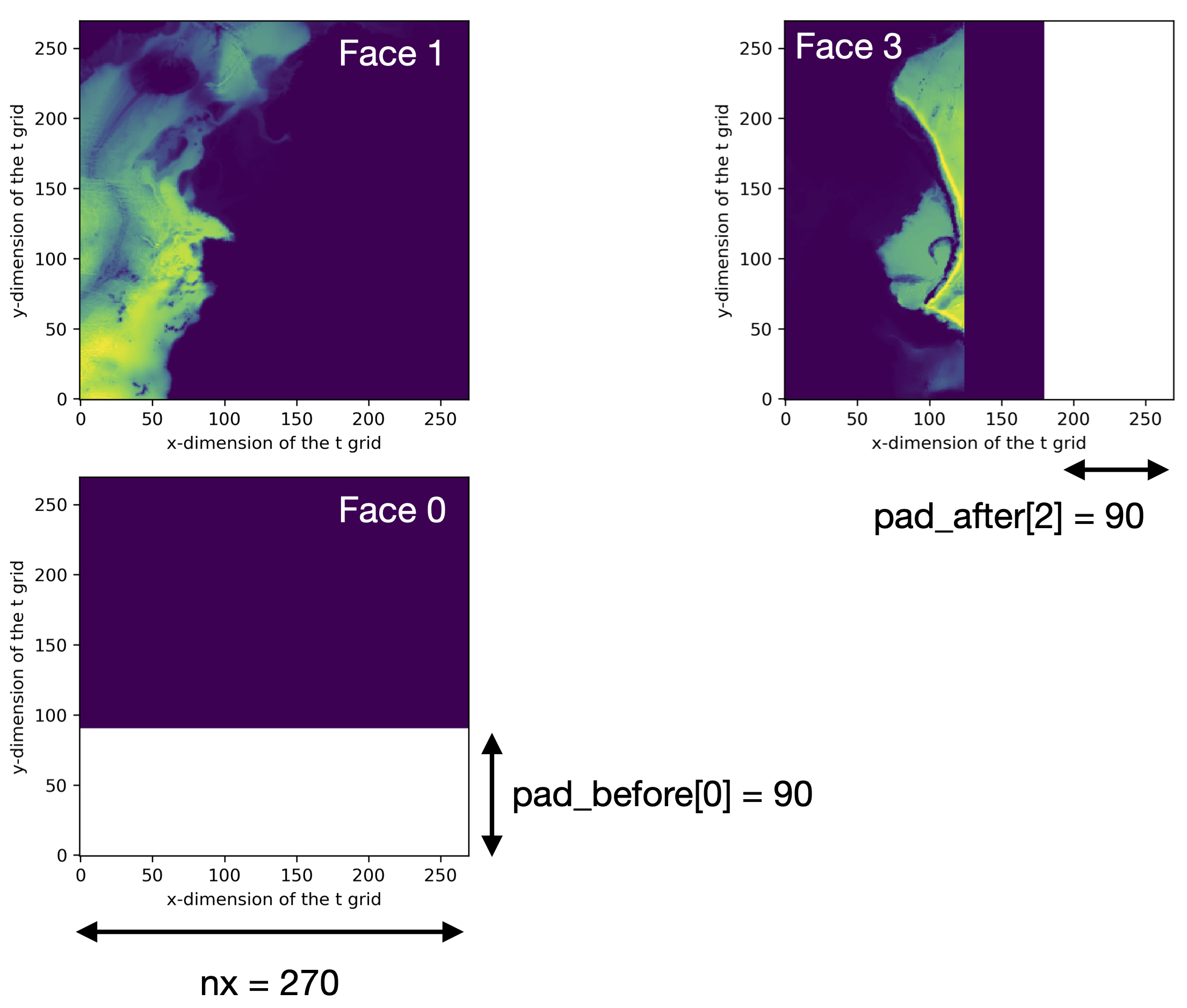
Left: faces 0 and 1 live on facet 0, as shown by _facet_strides.
This facet has an expected shape of
(2* nx , nx) = (540,270) as determined by _facet_shape.
The data shape is only (450,270), however, as shown in color.
To make two nx x nx tiles, the facet must be padded with a
(90,270) array, shown in white.
On this facet, reshape = False, so the j dimension is padded.
Right: face 3 lives on facet 2, and the expected data shape would
be (nx , nx) = (270,270), but the data only cover
(270,180), shown in color.
Therefore, the data are padded with an array of size (270,90),
shown in white, and this is padded to the i dimension
since reshape = True for this facet.